Kernel Density Estimation
Spatial Analysis
The visualization of GPS fixes as individual tracks is a powerful tool in movement ecology and conservation. Yet, when it comes to many individuals and long observation periods there are limitations. The detection of accumulations and frequently used regions can be deceiving when inferred from individual tracks. As patterns are scattered over time approaches are required that enable a viewpoint which integrates over both time intervals and spatial preferences.
Notes on the Firetail algorithm
For this purpose, numerous algorithms have been developed that accumulate locations of tracking data and estimate the likelihood of occurrence of individuals or species from sampled locations. Kernel Density Estimation (KDE) is among the most widely used tools in this regard.
A kernel in general may be seen as a measure of similarity among to locations (vectors) and thereby define a region of influence for a measurement. The size of this region is reflected by the kernel bandwidth, which is a parameter to KDE algorithms.
Firetail implements a fast and flexible box-filter approximation algorithm of gaussian convolution following Getreuer 2013 [1].
It features
- an adaptive resolution based on the induced areal extent of the GPS fixes
- bandwidth estimation from detected path characteristics
- inclusion/exclusion of selected individuals
- time window restrictions
- on-the-fly preview and computation for moderately sized data
- contour map visuals (95, 85, 50, 10 pct levels)
- resolution control
In Firetail, the bandwidth parameter can be controlled indirectly. Focussing the interactive use case the requirements of the current set of selected data are analyzed and a bandwidth scaling can be set that governs the bandwidth for a wide range of areal extents and data characteristics.
For larger datasets or long time extents resolutions other than preview may not be suited for interactive handling.
Rendering the KDE map as a video could be sensible depending on your use cases.
KDE computation
To show a quick Kernel Density Estimation
- open a project that features GPS fixes for one or more individuals
- select a subset of individuals you wish to analyze (or select all of them)
- choose
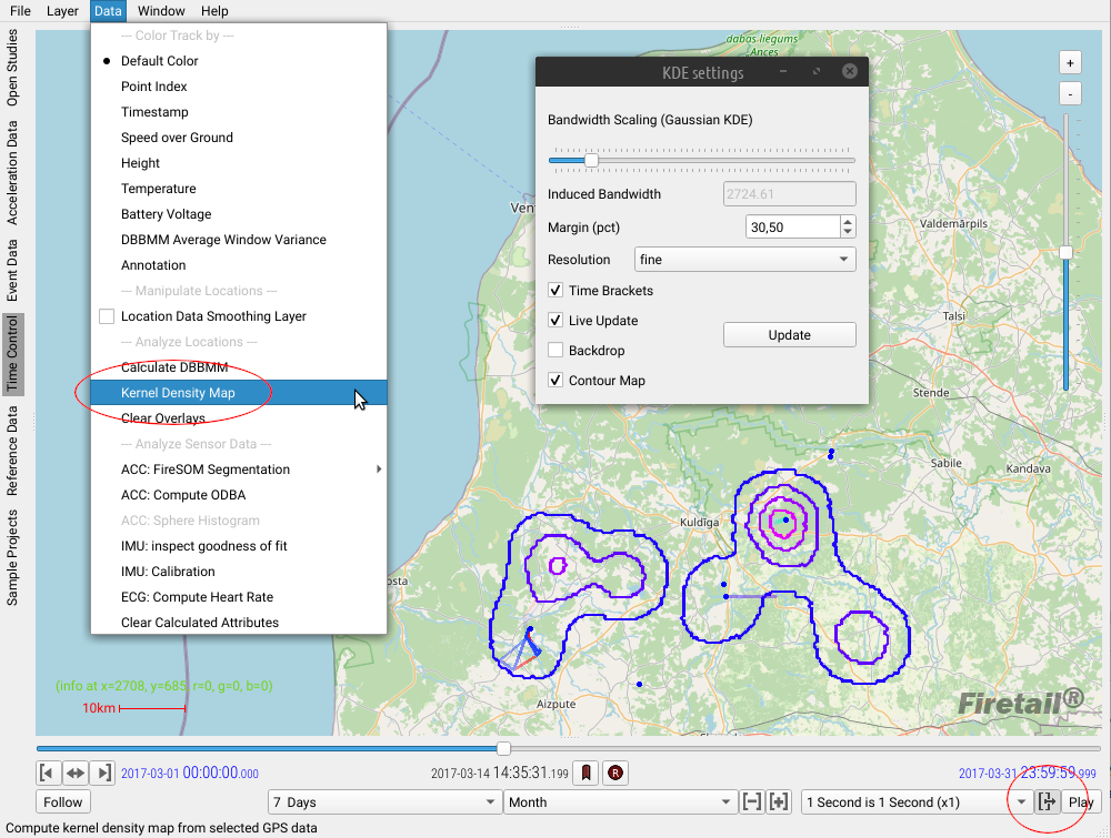
Data > Location and GPS > Kernel Density Map - The KDE control window will appear. Click
Updateto show the map in the main viewport.
In case the density map is covered by individual’s paths try to set the visible track interval to a lower value, e.g. a few hours.
KDE parameters
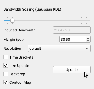
As discussed above, the bandwidth scaling setting will control the bandwidth with respect of the characteristics of the selected (subset of) data for both contour and KDE heatmaps. The Induced Bandwidth refers to the internally used bandwidth of the algorithm.
For some settings, the extent of contours or the heatmap may require an additional margin around the analyzed region to avoid hard cutoffs. Increase the Margin (pct) in this case.
The Resolution will influence the box filter width and height. A higher resolution will show more details in the KDE map as it may also allow for a smaller bandwidth. The required resolution depends on the dataset density and its spatial extent, but there is a tradeoff with interactive usage (see Live Update).
Checking Time Brackets will limit the computation of the KDE map to the currently selected time brackets in the main time control. In this way it is possible to compute a KDE map for a day, a week or any given custom range. This is particularly powerful when used in combination with a selected subset of individuals, e.g. via Firetails bookmarking mechanism.
Check Live Update to immediately recompute the map upon any change of parameters and when adapting the time brackets of the main time control. By shifting the brackets you will receive time-frame estimations for the selected locations (and individuals).
Combine this feature with the (Firetail 10) feature shift brackets while playing to recompute the map when replaying (Play) the dataset.

This will shift the selected time interval and recompute incremental updates of the KDE map along the time axis. The replay speed setting can be used to control how far the interval is shifted (per computed frame).
Toggle Backdrop to show a transparent grey frame around all currently active locations as well as the additional margin.
References
[1] Getreuer, P. A survey of Gaussian convolution algorithms. Image Processing On Line, 2013, 2013. Jg., S. 286-310.