Acceleration annotation

Annotation of acceleration data is increasingly important for a wide range of projects. Firetail provides you with a set of tools for manual and machine learning assisted (FireSOM) annotation. You can rapidly annotate

• Movebank individuals
• Movebank tags
• Movebank deployments

Core concepts

Firetail features layers as highest level of organisation. A layer can hold arbitrary many categories. Each category resides on one specific layer.

A burst (see also Burst vs. continuous recording) can be assigned to one or more categories.

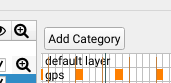
Add new categories

To add a new category press Add Category above the acceleration window

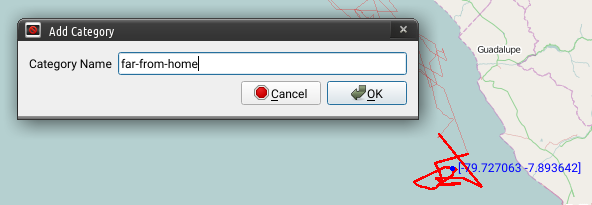
Assign a name to the category

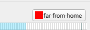
The category will show up above the acceleration window

Save and Load Annotation Categories

Annotation is usually a process done as a team to ensure consistency to have the possibility to check for inter-annotator agreements. Sharing a common set of annotation categories is crucial.

With Firetail you can save the current set of categories and layers. File > Annotations > Export Annotation Categories.

The resulting file can be shared and reimported. To add the categories to your current project, use File > Annotations > Import Annotation Categories.

Working with external annotations

Starting from version 9 Firetail introduces a simple yet powerful exchange format for annotations.

You can import multiple external annotation files. This allows you to

• show gold standards alongside with predicted annotations
• interpret reference data in the context of FireSOM predictions
• compare multiple predictions
• merge annotations from distinct sources

and much more.

Export/Import annotations

Caveat: Export/Import must not be confused with File > Save Annotations Saving causes the data to be saved along with your project. Export is designed to share annotations with peers or process external annotation resources.

To export annotations from Firetail use File > Annotations > Export Annotations. Select a filename of your choice and confirm your selection.

To import annotations use File > Annotations > Import External Annotations. Choose a csv annotation file and confirm your selection.

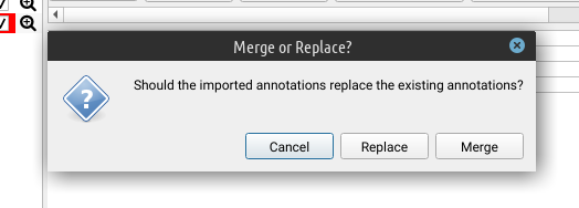
You will be asked about the procedure.

1. Replace: existing annotation layers will be replaced by the annotation file
2. Merge: layers and categories are merged with the existing annotation

The Firetail annotation exchange format

The current exchange format is contains comma-separated values as follows. The following sample shows the required header columns (UTF8 csv) and few sample categories across several layers

category, layer, start-timestamp, end-timestamp
"in", "default layer", 2012-06-01 08:20:00.000, 2012-06-03 21:21:10.000
"out", "default layer", 2012-06-15 16:22:03.000, 2012-06-15 23:27:30.000
"foo", "default layer", 2012-06-16 00:50:01.000, 2012-06-18 22:02:02.000
"bar", "flying", 2012-06-16 23:51:01.000, 2012-06-18 23:55:02.000
"bar", "flying", 2012-06-16 23:56:01.000, 2012-06-18 23:57:02.000

Each line one annotation category mapped onto a layer. category and layer are string types, whereas the timestamp should be an ISO timestamp with 3 ms digits.

If external resources do not feature a layer concept, the “default layer” can be assigned.

Firetail will gradually be extended with specific converters/import filters for external annotation formats. If you feel that a format is sufficiently important for many users please don’t hesitate to contact us!

Currently, the tag/individual/deployment information is not saved along with the data. The reason is simply that external tools are not aware of movebank conventions while grouping (layering) and category assignments with a distinct start and end are generic concepts. Exported data must not be mistaken for a complete snapshot including all required meta-information.

Make sure to include sufficient information in your filename structure to properly map your data to the respective tags or individuals.

Assign a category to a region

Once you have defined categories, you can use the selection mechanism described here to define regions that you’d like to annotate with one of your categories.

1. Select a region within the bursts or the map
2. Press on the category you want to assign this region to

The newly assigned category will be shown in a row/layer above the acceleration data.

Each category can be assigned to a single layer (visual group shown as a single row of data).

Note that overlapping categories shown in a single layer are possible, yet may not be visually sensible.

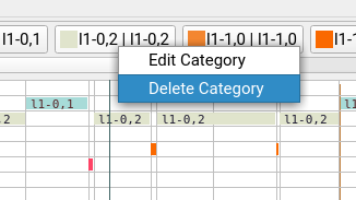
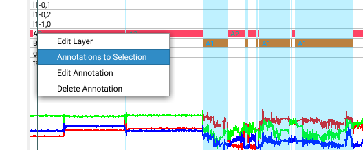
Right-clicking a category will yield a popup-menu for:

• category modification
• annotation deletion

Saving Annotations and Removing a category

You can remove existing categories via right-clicking on the respective category and select delete category. You are prompted that all annotations contained will be lost. There is currently no undo for this, so make sure to use

File > Save Annotations

to save the current state.

Expert hint: the annotation resides in the respective $USER/movebank_downloads/study_<num> folder as annotation2.csv (to ensure compatiblity with AccelerationViewer, this will likely change in future versions). Make sure to include this folder in your regular backup procedure

FireSOM: Machine-learning assisted acceleration segmentation

When working with acceleration data manual annotation of large-scale data may be time-consuming or near-impossible. Via Data > Acc: FireSOM Segmentation you can trigger Firetail’s automated segmentation algorithm FireSOM.

IMPORTANT: Firetail’s annotation features are activated when loading data via Download Movebank by ID/Tag/Deployment. Your annotation is saved locally (on your machine) along with the downloaded data.

Introduction to FireSOM

In addition to GPS fixes modern animal tags can provide high-resolution acceleration data measuring relative movement changes with respect to gravity in multiple, typically three (XYZ), axes. Commonly, the data is recorded as bursts. In this context, a burst is a sequence of measurements that is consecutively recorded at a fixed frequency for a limited amount of time. The burst length can range from few seconds to several minutes depending on the research context or dynamic tag settings.

The FireSOM algorithm as implemented in Firetail is an assistive system designed to annotate burst data by clustering bursts into abstract categories based on their overall similarity.

Machine learning algorithms share the idea to estimate data similarity via encodings of user-selected features rather than by comparing raw data. In FireSOM, each burst is first encoded as a vector of features. For simplicity, the user can select feature groups rather than single features. Selecting a group would then append all induced features to the feature vector of each burst.

To cluster similar bursts, FireSOM employs a self-organizing map (SOM, also referred to as Kohonen map [1]). A SOM is a 2-dimensional grid of (weighted) nodes. Each node represents a potential cluster/category. Placing bursts on the map (referred to as training) adapts the map structure (the node weights) to the dataset. After the training all recorded bursts are placed in the cluster that resembles its characteristic vector best. Bursts with similar features are located spatially close on the map or within the same node. They are assigned the same category.

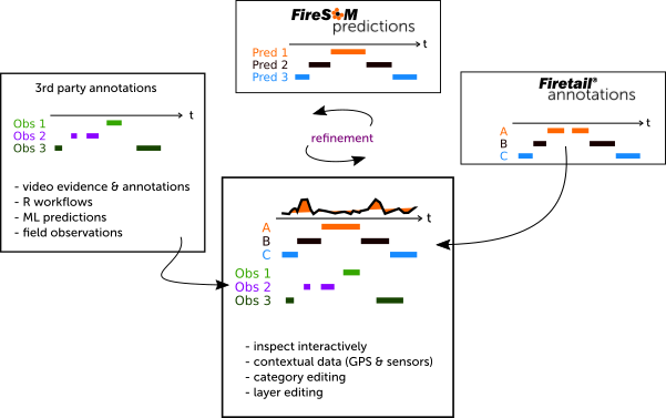
The initial result is an assignment of an abstract category to each burst. This can be visualized by annotation layers above the raw acceleration data (one layer per category). Abstract categories can then be analyzed in a GPS and sensor data context and assigned to known behavioral categories. By overlaying observation data or gold standards the validity of the predicted categories can be analyzed.

FireSOM can refine predicted categories via second layer predictions (re-train a category), merging of categories that are very similar and discard categories. This iterative refinement can be used to annotate complete datasets and also transfer results by using pre-trained models for the prediction of other tags, individuals or deployments.

FireSOM - Overview of the core algorithm steps

1. calculate a set of user-selected features for each burst
2. normalise (standardization) extracted features
3. train the FireSOM (self-organizing map) using the bursts mapped into feature space
4. assign each burst to a category

Video Tutorial

Here you can find a video tutorial on FireSOM, see below for more details

How to choose the map size?

The map size can be selected freely and must be adapted to the number of distinct behavioral categories. While more categories require more space on the map (more nodes), a large map requires more training data. Complex data patterns may require more nodes to reflect subtle changes in the data.

Start with as few as 9 nodes (a 3x3 map) and run FireSOM with basic statistic features enabled. This will likely separate active from inactive patterns. Some categories cover a too broad range of patterns (multiple behaviors). Move affected categories to a separate layer and use Annotations to Selections to refine these categories by restricting a second iteration of FireSOM on this selection.

Some datasets may require larger map sizes and more refinement steps. The model dimension determines the number of predicted categories. For a 4x5 sized map you’ll retrieve a maximum of 20 categories. Empty categories are deleted.

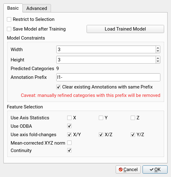
Model Constraints

Width: the number of horizontal nodes, we suggest to use at least 3 depending on the complexity of data patterns

Height: the number of vertical nodes, we suggest to use at least 3 depending on the complexity of data patterns

Annotation Prefix: Each predicted category will be prefixed with this string

Clear existing Annotations with the same Prefix: Any previous annotation with this prefix will be removed. Rename auto-predicted categories to avoid data loss.

Feature Groups

For simplicity, the user can select groups of features rather than single features. Selecting a group would then append all induced features to the feature vector of a burst. The following groups are available:

Axis Statistics: distribution statistics, each axis Basic features that encode per-axis statistics, in particular the maximum, minimum, median and 25%/75%-quantiles of a burst. We refer to this as canonical encoding. Specific axis may govern specific behavior (Y axis: upside down, X: forward, Z: shifting).

ODBA: overall dynamic body acceleration encoded as a feature, all axes The ODBA value with respect to the burst mean constitutes a single-value feature reflecting the energy usage of the burst.

axis fold-changes: distribution statistics for the log-2 fold-changes, pairwise axes The ‘axis fold-changes’ will compute the log-2 fold-changes among selected axes and then compute distribution statistics. Pairwise relations among axes may hint at complex movements.

mean-corrected norm: add the mean-corrected norm value for each burst The ‘mean corrected norm’ computes a normalized length for each recorded sample vector and computes canonical distribution statistics. The feature reflects an overall direction bias.

continuity: add a measure of sum of changes The absolute sum of changes that occur within a burst provides a single-valued feature reflecting the degree of movement in a burst. It resembles a non normalized flavor of ODBA.

Click OK to train a model and see your results as new layers in the acceleration window.

Inspecting the model

While it is easy to train a model in Firetail, there is no intrinsic way for Firetail to decide on model quality.

Inspecting a predicted model is crucial

Firetail provides you with a lot of context that makes it easier to interpret the predictions and would also allow to overlay annotations as gold standards, 3rd party predictions, or observational data. But also location data data and sensor data may hint to prediction quality.

Overall, the model is based on the similarity of two bursts in feature space, so similar patterns should be assigned to identical or nearby categories. Neighborhood is defined in a tabular row-column sense, i.e node (1,4) is a direct neighbor of (1,3), (1,5), (0,4) and so on.

Think of patterns in terms of activities like rest, running or feeding. The more categories you predict the more behavioural complexity can be detected. For increasingly many categories it may become necessary to join predictions via layers to group similar categories.

Start simple

Therefore, start by training a simple model with dimension 3 by 3 and few features. You can easily train a quick model as a preview or even experiment with how well a single feature works for discrimination of visual patterns or regions of known behaviour.

Increase complexity if required

An increasing number of features means there is more freedom to discriminate bursts. The result model will be harder to interpret though. Incrementally increase model complexity and add features when two regions you deem dissimilar are placed in the same category.

Refine using local models

If the data features local specificities it makes sense to run the segmentation on a selection.

Make sure that at least a few hundred bursts are selected to avoid a poorly fitted model.

In this context, the option Restrict to Selection must be enabled.

The algorithm will predict categories only for selected bursts. Choose a distinct model prefix to make sure to maintain both global and local predictions.

Refine specific categories

Right clicking on an annotation layer allows you to select annotatated regions by choosing “Annotations to Selections”.

This leads to a powerful workflow:

1. select regions that could not be segmented properly by the initial, coarse model
2. make sure that the regions to be refined are selected
3. re-run FireSOM using Restrict to Selection and a new model prefix
4. evaluate the local model via merge/delete semantics as discussed below

Assign, Rename and group

The machine-assigned group names cannot magically predict “running”, “feeding” or “flying”. Screen the predicted categories visually and in their best possible context to assign a category to a possibly preliminary behaviour. Repeated

• application of the segmentation
• changes in parameters and
• successive joining of categories into layers
• refinement of coarse categories
• deletion of superfluous categories

will lead to sensible annotations for a complete dataset.

Saving a model

You can save a trained model for later use on another dataset or selection. This provides a very powerful way to avoid the inclusion artifacts or to build more specific models. The core idea is to sort bursts into buckets defined in another context. Therefore, this strategy should work best on similar input data, although there is no technical constraint keeping the user from applying models cross-species or across tag-types.

A common use case is to save global and refined models for one dataset (see refinement) and then re-apply the models on another dataset.

An appropriate setup could also help to enforce consistency checks and enable in-depth validation.

The key steps are:

1. check Save Model after Training
2. set the required parameters and features
3. press OK to train the model
4. select a file to save the training state

A model is a json file that includes required map-weights, parameter settings and the selection of features. The application of this model on different data requires the same parameters and features.

Using a previously trained model

To apply a pre-trained model:

1. load the model via Load Trained Model
2. optional: choose a new prefix to avoid losing existing annotations
3. note that the feature selection and most parameters will be deactivated
4. press OK

The (selected) bursts are then classified using the pre-defined model.

General

Combine the concepts of

• selecting regions
• selecting by layer content
• merge categories into layers
• delete categories
• train local models
• train global models
• vary parameters
• vary features
• predict locally

to build models specific to your use-case.

References

[1] Kohonen, Teuvo (1982). “Self-Organized Formation of Topologically Correct Feature Maps”. Biological Cybernetics. 43 (1): 59–69. doi:10.1007/bf00337288. S2CID 206775459